The canopy data model
The Field object
Canopy stores data in a self-describing container called a Field. A Field is meant to represent a spatio-temporally varying DGVM diagnostic or output (e.g., annual GPP, stored carbon, LAI…). Each quantity may be further disaggregated into layers (e.g., GPP can be disaggregated into PFTs, carbon storage into different carbon pools…)
A Field object consists of:
A pandas DataFrame with a spatio-temporal index to store the field’s data
A
Gridobject describing the grid associated with the dataA metadata dictionary
A history dictionary
Methods for basic data slicing and reduction.
To create a Field, the pandas DataFrame and the associated grid must be supplied. For the Field object to be successfully instantiated, it must fulfill the specifications below, and the data and the grid must be compatible.
The DataFrame
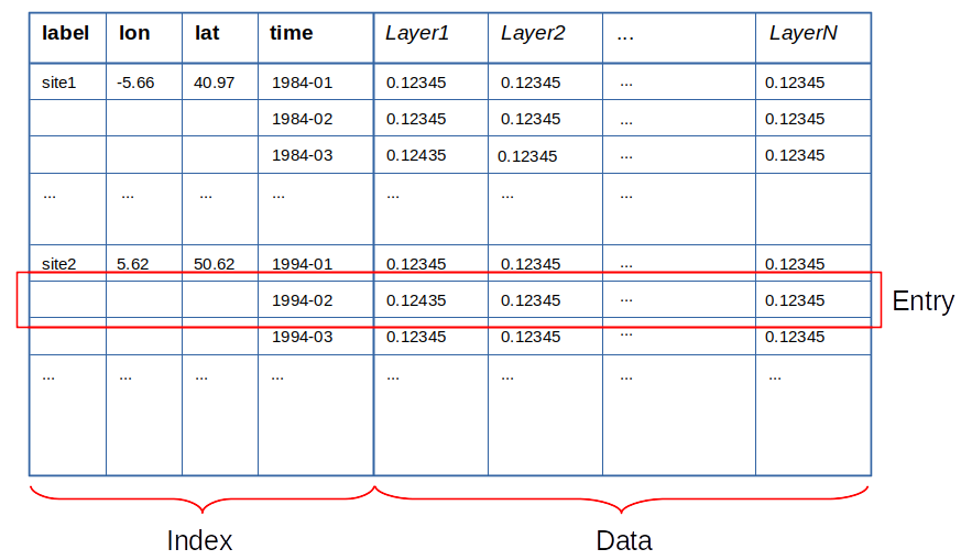
The data table is a pandas DataFrame containing the spatio-temporal indexed data.
Layers are stored as columns. The column identifiers (names) must be of str type.
The index must contain at least one time level of pandas PeriodIndex type.
It may additionally contain one or two spatial levels (e.g. lon and lat), of float type.
One additional, redundant label level is allowed, but not required, for site-based data (or, in general, any data associated to an unstructured grid).
The index levels can therefore have one of the following forms:
[label, x_1, x_2, time]: Fully spatio-temporal site-based data, with a _redundant_ index level label.
[x_1, x_2, time]: Fully spatio-temporal data, with two spatial dimensions (x_1 and x_2 could be, e.g., lon and lat).
[x_1, time]: Spatio-temporal data, dimension x_2 has been reduced.
[x_2, time]: Spatio-temporal data, dimension x_1 has been reduced.
[time]: Time series. It can represent purely temporal data or data whose spatial dimensions have both been reduced.
Note
Entry refers to a single spatio-temporal location (a row of the table).
Note
Currently, canopy does not support a vertical coordinate nor subgrid indexing (but it will in the future).
The Grid object
Grid objects describe different types of grids. These are implemented as subclasses of the abstract base class Grid (described below). Instances of a Grid subclass provide all the necessary information to perform spatial reduction operations (grid operations or _gridops_) associated to that grid type.
Currently, canopy comes with two grid types and their associated operations:
lonlat: describes a standard geographical (longitude-latitude) grid. The grid spacing is constant, but can be different for each axis.sites: describes an unstructured grid, such as the one associated to a collection of sites.
There is a special type of grid, empty, which is used for pure time series (no spatial dimensions).
All grids are derived from the abstract base class Grid, and override the following methods:
Grid.from_frame()(class method): constructs aGridobject from a pandas DataFrameGrid.validate_frame(): checks that the grid describes the data contained in the supplied DataFrame correctly (i.e., if the frame’s index is compatible with the grid).Grid.crop(): returns a croppedGridof the same type, orGridEmptyif the supplied dataframe is empty or outside the grid’s domain.Grid.reduce(): returns a reducesGridof the same type, orGridEmptyif both axes are reduced.Grid.is_compatible(): Checks for compatibility of two grids, i.e., if two grids can be added together. All grids are compatible with the typeGridEmpty. As an example, twoGridLonLatgrids are compatible if the grids extended to cover the globe overlap perfectly (i.e., they are subsets of the same global grid).Grid.__add__(): returns the sum of twoGridobjects, which is anotherGridobject. AddingGridEmptyto a grid object simply returns a deep copy of the object.
Additionally, all subclasses define the following class attributes:
_grid_type: str: The name under which the grid subclass will be registered in the grid registry.
_xaxis: SpatialAxis: Named tuple of type
SpatialAxisdefining the grid’s X axis attributes._yaxis: SpatialAxis: Named tuple of type
SpatialAxisdefining the grid’s Y axis attributes._xaxis_key: Short key to refer to the grid’s X axis (e.g. in grid operations).
_yaxis_key: Short key to refer to the grid’s Y axis (e.g. in grid operations).
The derived class can override the Grid base class __init__() method. However, the overriden __init__() must still call the base class’ __init__() by using the super() function.
Creating a Field
In order to gain insight into the structure of a Field object, we will create one from scratch. We encourage you to try this example on your own. This is, of course, a dummy example with randomly generated data. Normally, the Field is created by data-reader functions from model output files or from an observational dataset. See Reading files and Data sources.
First we need a multi-indexed DataFrame. Let’s create one purporting to hold plant annual transpiration (in mm) by PFT, in mm, for a small 2x2 gridcells domain between 1999 and 2001 on a lonlat grid.
import pandas as pd
import numpy as np
import canopy as cp

pfts = ['Conifer', 'Broadleaf', 'Grass', ]
years = [pd.Period(year=x, freq='Y') for x in [1999, 2000, 2001]]
lons = [13.25, 13.75]
lats = [40.75, 41.25]
index = pd.MultiIndex.from_product([lons, lats, years], names=['lon', 'lat', 'time'])
np.random.seed(10)
data = 200*np.random.random(len(index)*len(pfts)).reshape([len(index), len(pfts)])
data = pd.DataFrame(data, index=index, columns=pfts)
print(data)
                     Conifer   Broadleaf       Grass
lon   lat   time
13.25 40.75 1999  154.264129    4.150390  126.729647
            2000  149.760777   99.701402   44.959329
            2001   39.612573  152.106142   33.822167
      41.25 1999   17.667963  137.071964  190.678669
            2000    0.789653  102.438453  162.524192
            2001  122.505213  144.351063   58.375214
13.75 40.75 1999  183.554825  142.915157  108.508874
            2000   28.434010   74.668152  134.826723
            2001   88.366635   86.802799  123.553396
      41.25 1999  102.627649  130.079436  120.207791
            2000  161.044639  104.329430  181.729776
            2001   63.847218   18.091870   60.140011
Now, let’s create a Grid object associated with this data. The grid specifications can be inferred from the DataFrame of interests by invoking the Grid.from_frame() constructor as follows:
grid = cp.grid.get_grid('lonlat').from_frame(data)
print(grid)
Longitude:
13.25 to 13.75 (step: 0.5)
Latitude:
40.75 to 41.25 (step: 0.5)
Finally, we construct the Field object. It looks like not much is going on, but the Field constructor will verify the DataFrame to ensure that the data conforms to the canopy data model described above.
# Annual transpiration
aaet = cp.Field(grid, data)
print(aaet)
Data
----
name: [no name]
units: [no units]
description: [no description]

Grid: lonlat
------------
Longitude:
13.25 to 13.75 (step: 0.5)
Latitude:
40.75 to 41.25 (step: 0.5)

Time series
-----------
Span: 1999-01-01 00:00:00 - 2001-12-31 23:59:59.999999999
Frequency: Y-DEC

History
-------
To examine the Field’s data, one can use:
print(f"Field's layers: {aaet.layers}")
print("Field's data:")
print(aaet.data)
Field's layers: ['Conifer', 'Broadleaf', 'Grass']
Field's data:
                     Conifer   Broadleaf       Grass
lon   lat   time
13.25 40.75 1999  154.264129    4.150390  126.729647
            2000  149.760777   99.701402   44.959329
            2001   39.612573  152.106142   33.822167
      41.25 1999   17.667963  137.071964  190.678669
            2000    0.789653  102.438453  162.524192
            2001  122.505213  144.351063   58.375214
13.75 40.75 1999  183.554825  142.915157  108.508874
            2000   28.434010   74.668152  134.826723
            2001   88.366635   86.802799  123.553396
      41.25 1999  102.627649  130.079436  120.207791
            2000  161.044639  104.329430  181.729776
            2001   63.847218   18.091870   60.140011
Notice that our created-by-hand Field does not yet have metadata. In normal canopy workflow, the metadata is added upon reading from disk by the reader function or the Source object (see Basic data manipulation), as long as the data source is registered. Metadata can be added or reset manually as follows:
# Fails because the entry 'name' already exists by default in every Field.
#aaet.add_md('name', 'aaet')
# For existing entries, like the three default ones, we use Field.set_md()
aaet.set_md('name', 'aaet')
aaet.set_md('description', 'Annual transpiration by PFT')
aaet.set_md('units', 'mm')
# We can add any metadata we want with Field.add_md()
aaet.add_md('scenario', 'SSP1-2.6')
# We can also manually add entries to the history log
aaet.log('Field created manually with bogus data')
print(aaet)
Data
----
name: aaet
units: mm
description: Annual transpiration by PFT
scenario: SSP1-2.6

Grid: lonlat
------------
Longitude:
13.25 to 13.75 (step: 0.5)
Latitude:
40.75 to 41.25 (step: 0.5)

Time series
-----------
Span: 1999-01-01 00:00:00 - 2001-12-31 23:59:59.999999999
Frequency: Y-DEC

History
-------
2025-05-12 19:20:48: Field created manually with bogus data