Basic data manipulation
Reading files
The basic way to read a data file into a Field object is by using the Field.from_file() class method as follows:
import canopy as cp
cpool = cp.Field.from_file('/path/to/output/cpool.out.gz', file_format='lpjg_annual', grid_type='lonlat', source='lpjguess:cpool')
This reads the file cpool.out.gz, located at /path/to/output/.
The
file_formatargument specifies the format of the file (e.g.,lpjg_annual,lpjg_monthly,fluxnet2015…)The
grid_typeargument specifies the associated grid (e.g.,lonlat,sites…)The optional
sourceargument specifies the metadata to retrieve. The format for this argument issource:field(e.g.,lpjguess:cpool,lpjguess:anpp…)
Note
LPJ-GUESS output files can be in plain text or gzipped; the reader will manage this automatically.
The format lpjg_annual and the grid type lonlat are actually the default, so the line below accomplishes the same task:
cpool = cp.Field.from_file('/path/to/output/cpool.out.gz', source='lpjguess:cpool')
Printing the field gives us some basic information about it:
print(cpool)
Data
----
name: C pools
description: Ecosystem carbon mass by pool
units: kgC m⁻²
file format: LPJ-GUESS: common output (annual)
original file: /path/to/output/cpool.out.gz

Grid: lonlat
------------
Longitude:
-26.25 to 34.75 (step: 0.5)
Latitude:
35.25 to 71.75 (step: 0.5)

Time series
-----------
Span: 1850-01-01 00:00:00 - 2014-12-31 23:59:59.999999999
Frequency: Y-DEC

History
-------
[1] 2025-05-08 20:27:57: Data read from /path/to/output/cpool.out.gz
Data sources
A data Source object provides a convenient way to access data. The source can be a directory with model output or measurement data:
import canopy as cp
my_run = cp.get_source('/path/to/output/', 'lpjguess')
# Print available fields
print(my_run)
Source: LPJ-GUESS
Path: /path/to/output

L  M  Field       Description                                            (units)
-----------------------------------------------------------------------------------------
      aaet        Annual actual evapotranspiration by PFT                (mm year⁻¹)
      agpp        Annual gross primary productivity by PFT               (kgC m⁻² year⁻¹)
      anpp        Annual net primary productivity by PFT                 (kgC m⁻² year⁻¹)
      cflux       Annual carbon flux by pool                             (kgC m⁻² year⁻¹)
      cmass       Carbon mass in the vegetation pool by PFT              (kgC m⁻²)
      cpool       Ecosystem carbon mass by pool                          (kgC m⁻²)
      cton_leaf   Leaf carbon to nitrogen ratio by PFT                   (kgC/kgN)
      dens        Number of individuals per unit area, per PFT           (m⁻²)
      doc         Dissolved Organic Carbon                               (kgC ha)
      fpc         Fraction of modeled area covered by vegetation by PFT  (1)
      lai         One-sided leaf area per unit of modeled area by PFT    (1)
      nflux       Nitrogen flux by different processes                   (kgN ha year⁻¹)
      ngases      Flux of nitrogen gases from soil or fire               (kgN ha year⁻¹)
      nmass       Nitrogen mass stored in the vegetation by PFT          (kgN ha)
      npool       Ecosystem nitrogen mass by pool                        (kgN ha)
      nsources    Nitrogen sources by type                               (kgN ha year⁻¹)
      soil_nflux  Nitrogen flux from the soil by gaseous species         (kgN ha year⁻¹)
      soil_npool  Nitrogen storage in the soil by pool                   (kgN ha)
      tot_runoff  Total water runnoff by PFT                             (mm year⁻¹)
A field can be loaded from disk with the Source.load_field() method. The field will appear as loaded (L):
my_run.load_field('cpool')
print(my_run)
Source: LPJ-GUESS
Path: /path/to/output

L  M  Field       Description                                            (units)
-----------------------------------------------------------------------------------------
      aaet        Annual actual evapotranspiration by PFT                (mm year⁻¹)
      agpp        Annual gross primary productivity by PFT               (kgC m⁻² year⁻¹)
      anpp        Annual net primary productivity by PFT                 (kgC m⁻² year⁻¹)
      cflux       Annual carbon flux by pool                             (kgC m⁻² year⁻¹)
      cmass       Carbon mass in the vegetation pool by PFT              (kgC m⁻²)
      cpool       Ecosystem carbon mass by pool                          (kgC m⁻²)
✓     cton_leaf   Leaf carbon to nitrogen ratio by PFT                   (kgC/kgN)
      dens        Number of individuals per unit area, per PFT           (m⁻²)
      doc         Dissolved Organic Carbon                               (kgC ha)
      fpc         Fraction of modeled area covered by vegetation by PFT  (1)
      lai         One-sided leaf area per unit of modeled area by PFT    (1)
      nflux       Nitrogen flux by different processes                   (kgN ha year⁻¹)
      ngases      Flux of nitrogen gases from soil or fire               (kgN ha year⁻¹)
      nmass       Nitrogen mass stored in the vegetation by PFT          (kgN ha)
      npool       Ecosystem nitrogen mass by pool                        (kgN ha)
      nsources    Nitrogen sources by type                               (kgN ha year⁻¹)
      soil_nflux  Nitrogen flux from the soil by gaseous species         (kgN ha year⁻¹)
      soil_npool  Nitrogen storage in the soil by pool                   (kgN ha)
      tot_runoff  Total water runnoff by PFT                             (mm year⁻¹)
The field can be accessed through the dot (.) operator. If the field held in the Source object is modified, it will be indicated under M:
# Create a new field 'cpool_av' by averaging in space.
# This doesn't modify the original field
cpool_av = my_run.cpool.reduce_grid('av')

# Average the original field in place (it will appear as modified in the Source object)
my_run.cpool.reduce_grid('av', inplace=True)
print(my_run)
Source: LPJ-GUESS
Path: /home/belda-d/data/pyguess_test_data/europe_LR_100p/output/

L  M  Field       Description                                            (units)
-----------------------------------------------------------------------------------------
      aaet        Annual actual evapotranspiration by PFT                (mm year⁻¹)
      agpp        Annual gross primary productivity by PFT               (kgC m⁻² year⁻¹)
      anpp        Annual net primary productivity by PFT                 (kgC m⁻² year⁻¹)
      cflux       Annual carbon flux by pool                             (kgC m⁻² year⁻¹)
      cmass       Carbon mass in the vegetation pool by PFT              (kgC m⁻²)
      cpool       Ecosystem carbon mass by pool                          (kgC m⁻²)
✓  ✓  cton_leaf   Leaf carbon to nitrogen ratio by PFT                   (kgC/kgN)
      dens        Number of individuals per unit area, per PFT           (m⁻²)
      doc         Dissolved Organic Carbon                               (kgC ha)
      fpc         Fraction of modeled area covered by vegetation by PFT  (1)
      lai         One-sided leaf area per unit of modeled area by PFT    (1)
      nflux       Nitrogen flux by different processes                   (kgN ha year⁻¹)
      ngases      Flux of nitrogen gases from soil or fire               (kgN ha year⁻¹)
      nmass       Nitrogen mass stored in the vegetation by PFT          (kgN ha)
      npool       Ecosystem nitrogen mass by pool                        (kgN ha)
      nsources    Nitrogen sources by type                               (kgN ha year⁻¹)
      soil_nflux  Nitrogen flux from the soil by gaseous species         (kgN ha year⁻¹)
      soil_npool  Nitrogen storage in the soil by pool                   (kgN ha)
      tot_runoff  Total water runnoff by PFT                             (mm year⁻¹)
Note
The names, descriptions, and units in the source-object-printout are those of the original fields. The source itself does not keep track of the modifications done inplace to a field; it only shows that the original field was altered.
Slicing data
Space- and time- slicing
The data can be sliced by invoking the Field.select_slice() (select slice) method, which takes a dictionary specifying the slices along each axis.
The spatial slices are specified as a tuple of numbers.
- The time axis slice is specified is also a tuple whose elements can be:
Python datetime objects.
ISO format date/time strings (e.g.
'2010-03-31').Integer values, which are interpreted as years.
# Spain bounding box: [9.5W - 3.5E] [35.5N - 44N]
cpool_spain = my_run.cpool.select_slice({'lon':(9.5,3.5),
                                         'lat':(35.5,44),
                                         'time'=(1901,2000)}
                                         )
print(cpool_spain)
Data
----
name: C pools
description: Ecosystem carbon mass by pool
units: kgC m⁻²
file format: LPJ-GUESS: common output (annual)
original file: /path/to/output/cpool.out.gz

Grid: lonlat
------------
Longitude:
-9.25 to 3.25 (step: 0.5)
Latitude:
35.75 to 43.75 (step: 0.5)

Time series
-----------
Span: 1901-01-01 00:00:00 - 2000-12-31 23:59:59.999999999
Frequency: Y-DEC

History
-------
[1] 2025-05-09 12:55:41: Data read from /home/belda-d/data/pyguess_test_data/europe_LR_100p/output/cpool.out.gz
[2] 2025-05-09 12:56:17: Sliced field along lon axis: (-9.5, 3.5).
[3] 2025-05-09 12:56:17: Sliced field along lat axis: (35.5, 44).
[4] 2025-05-09 12:56:17: Sliced field along time axis: ('1901-01-01', '2000-12-31').
Layer selection
To select layers, either the Field.select_layers() or square-bracket notation can be used. The argument can be the name of a layer or a list of names. To discard layers, use the Field.drop_layers() method:
print(f"Current field layers: {cpool_spain.layers}")

# Using select_slice to select the 'Total' carbon pool
cpool_tot = cpool_spain.select_slice('Total')
print(f"Just the 'Total' layer (select_layers method): {cpool_tot.layers}")

# Using square brackets to select the 'Total' layer
cpool_tot2 = cpool_spain['Total']
print(f"Just the 'Total' layer (using []): {cpool_tot.layers}")

# Selecting more than one layer:
cpool_nonveg = cpool_spain[['SoilC', 'LitterC']]
print(f"Layers of cpool_nonveg: {cpool_nonveg.layers}")

# Drop 'Total' layer
cpool_notot = cpool_spain.drop_layers('Total')
print(f"Layers of cpool_notot: {cpool_notot.layers}")
Current field layers: ['VegC', 'LitterC', 'SoilC', 'Total']
Just the 'Total' layer (select_slice): ['VegC', 'LitterC', 'SoilC', 'Total']
Just the 'Total' layer (using []): ['VegC', 'LitterC', 'SoilC', 'Total']
Layers of cpool_nonveg: ['SoilC', 'LitterC']
Layers of cpool_notot: ['VegC', 'LitterC', 'SoilC']
Reducing data
Spatial reductions
The data can be reduced along the spatial axes by invoking the Field.reduce_grid() method, which takes as arguments the grid reduction operation (gridop, one of av, sum), and the axis along which to perform the reduction (lat, lon, or both, the default value). The grid reduction operation will apply the appropriate geometrical factors corresponding to each grid type.
cpool_sum_lon = cpool_spain.reduce_grid('sum', 'lon') # Aggregate along the longitudinal axis
cpool_sum = cpool_spain.reduce_grid('sum') # Aggregate on both axes
cpool_av = cpool_spain.reduce_grid('av') # Average on both axes
print(cpool_av)
Data
----
name: C pools
description: Ecosystem carbon mass by pool
units: kgC m⁻²
file format: LPJ-GUESS: common output (annual)
original file: /path/to/output/cpool.out.gz

Grid: lonlat
------------
Longitude:
reduced (gridop = av)
Latitude:
reduced (gridop = av)

Time series
-----------
Span: 1901-01-01 00:00:00 - 2000-12-31 23:59:59.999999999
Frequency: Y-DEC

History
-------
2025-05-09 12:55:41: Data read from /home/belda-d/data/pyguess_test_data/europe_LR_100p/output/cpool.out.gz
2025-05-09 12:56:17: Sliced field along lon axis: (-9.5, 3.5).
2025-05-09 12:56:17: Sliced field along lat axis: (35.5, 44).
2025-05-09 12:56:17: Sliced field along time axis: ('1901-01-01', '2000-12-31').
2025-05-09 13:26:22: Spatial reduction: 'av', 'both'
Time reductions
Reductions along the time axis are applied through the Field.reduce_time() method. This method takes as arguments the time reduction operation (timeop, one of av or sum) and the frequency (freq) of the reduction, in the format nP, where n is an integer number, and P is a time period. For example, to average every 5 years, the freq argument would be the string 5Y.
# Time aggregation
cpool_timesum = cpool_spain.reduce_time('sum')

# Time average
cpool_tav = cpool_spain.reduce_time('av')

# Time average every 5 years
cpool_tav_5year = cpool_spain.reduce_time('av', '5Y')
print(cpool_tav_5year)
Data
----
name: C pools
description: Ecosystem carbon mass by pool
units: kgC m⁻²
file format: LPJ-GUESS: common output (annual)
original file: /path/to/output/cpool.out.gz

Grid: lonlat
------------
Longitude:
-9.25 to 3.25 (step: 0.5)
Latitude:
35.75 to 43.75 (step: 0.5)

Time series
-----------
Span: 1901-01-01 00:00:00 - 2000-12-31 23:59:59.999999999
Frequency: 5Y-DEC
Reduction: 'av'

History
-------
2025-05-09 12:55:41: Data read from /home/belda-d/data/pyguess_test_data/europe_LR_100p/output/cpool.out.gz
2025-05-09 12:56:17: Sliced 'lon': (-9.5, 3.5)
2025-05-09 12:56:17: Sliced 'lat': (35.5, 44)
2025-05-09 12:56:17: Sliced 'time': (1901, 2000)
2025-05-09 15:12:38: Time reduction: av, 5Y
Layer reductions
The method Field.reduce_layers() allows to create a new layer from two or more existing layers. The method accepts the following arguments:
redop: The reduction operation; currently one ofsum,av,maxLay,/.
layers: A list of layer names to be reduced.
name: The name of the new layer.
drop: A boolean indicating whether to drop the original layers (default:False).
print("Original data:")
print(cpool_spain.data)

# Calculate the Total C
layers = cpool_spain.layers # ['VegC', 'LitterC', 'SoilC', 'Total']
layers.remove('Total') # ['VegC', 'LitterC', 'SoilC']
cpool_spain.reduce_layers('sum', layers, name='TotalC2', inplace=True)

# Calculate the ratio of VegC to Total
cpool_spain.reduce_layers('/', ['VegC', 'Total'], name='VegC_ratio', inplace=True)
print("After layer reductions:")
print(cpool_spain.data)
Original data:
                    VegC  LitterC  SoilC   Total
lon   lat   time
-9.25 38.75 1901   3.779    1.046  4.305   9.130
            1902   3.717    1.087  4.299   9.102
            1903   3.648    1.112  4.307   9.067
            1904   3.755    1.064  4.308   9.127
            1905   3.824    1.078  4.307   9.209
...                  ...      ...    ...     ...
 3.25 43.75 1996  15.585    7.749  8.903  32.237
            1997  15.680    7.696  8.900  32.275
            1998  15.552    7.878  8.897  32.327
            1999  15.636    7.783  8.897  32.316
            2000  15.554    7.856  8.896  32.306

[30200 rows x 4 columns]
After layer reductions:
                    VegC  LitterC  SoilC   Total  TotalC2  VegC_ratio
lon   lat   time
-9.25 38.75 1901   3.779    1.046  4.305   9.130    9.130    0.413910
            1902   3.717    1.087  4.299   9.102    9.103    0.408372
            1903   3.648    1.112  4.307   9.067    9.067    0.402338
            1904   3.755    1.064  4.308   9.127    9.127    0.411417
            1905   3.824    1.078  4.307   9.209    9.209    0.415246
...                  ...      ...    ...     ...      ...         ...
 3.25 43.75 1996  15.585    7.749  8.903  32.237   32.237    0.483451
            1997  15.680    7.696  8.900  32.275   32.276    0.485825
            1998  15.552    7.878  8.897  32.327   32.327    0.481084
            1999  15.636    7.783  8.897  32.316   32.316    0.483847
            2000  15.554    7.856  8.896  32.306   32.306    0.481459

[30200 rows x 6 columns]
The RedSpec object
The RedSpec (Reduction Specification) class can hold information about a number of reduction operations, and can be passed to the Field.reduce() method. This can be used to, for example, apply the same slicing/reduction to a number of fields:
rs = cp.RedSpec(slices={'lat':(35.5,44),
                        'lon':(-9.5,3.5),
                        'time':(1901,2000)},
                gridop='av',
                axis='both',
                layers='Total')

aaet = my_run.load_field('aaet')
anpp = my_run.load_field('anpp')
agpp = my_run.load_field('agpp')

reduced_fields = []
for field in [aaet, anpp, agpp]:
    reduced_fields.append(field.reduce(rs))

for field in reduced_fields:
    print(field)
Filtering data
Use the Field.filter() method to extract rows from a Field object that match a boolean condition, expressed as a query string using layers.
# Load field
anpp = Field.from_file("/path/to/file/anpp.out")

# Keep only rows where 'Total' > 100
anpp_above5 = anpp.filter('Total > 0.5')

# In-place filtering with multiple conditions
anpp.filter('Total > 0.5 and Abi_alb < 0.3', inplace=True)
By default, Field.filter() removes non-matching entries, but you can keep them and set their values to NaN using fill_nan=True.
Note
See pandas documentation for DataFrame.query() for more details on the query string.
Operations on field layers
Arithmetic operations
The normal arithmetic operations can be applied to a field’s data.
The operands can either be two fields or a field and a scalar.
When combining two fields, their indices must match.
If both fields have the same number of layers, the operation is performed ‘element-wise’
If one of the fields has only one layer, the operation is performed ‘layer-wise’ (i.e. that one layer will be combined with all the layers of the other field).
Let’s illustrate this through an example. Here, agpp and anpp come from the same simulations and have the same index and number of layers. The - operation will subtract corresponding values of both fields.
import canopy as cp

agpp = cp.Field.from_file('/path/to/annual/gpp')
anpp = cp.Field.from_file('/path/to/annual/npp')

# Calculate respiration by subtracting npp from gpp
resp = agpp - anpp
If one of the fields has only 1 layer, the operation will be applied to all the other field’s layers, one by one. For example, we can select the ‘Total’ layer of a field, and divide all layers of the field by ‘Total’.
import canopy as cp

agpp = cp.Field.from_file('/path/to/annual/gpp')

# Calculate gpp as a FRACTION of the total:
agpp_frac_total = agpp / agpp['Total']
If one of the operands is a scalar, the operation will combine this scalar with all the values in the field.
import canopy as cp

agpp = cp.Field.from_file('/path/to/annual/gpp')

# Calculate gpp as a PERCENTAGE of the total:
# (divide by the total and multiply by 100)
agpp_perc_total = 100 * agpp / agpp['Total']
The apply method
The Field.apply() method can be used to apply numerical operations to a field or to selected layers. A basic call to Field.apply() takes two arguments, the operation to apply and the operand:
# Multiply all layers by two
anpp = anpp.apply("*", 2)

# Whoops! That was a mistake. Let's divide by two
anpp = anpp.apply("/", 2)
The operand can be a number, as in the example above, or the name of a layer, in which case the operation is applied element-wise:
# Let's express the field's values in percentage of the 'Total' layer:
anpp_percent = anpp.apply("/", "Total").apply("*", 100)
anpp_percent.set_md("units", "%")
Any operation can be applied to only selected layers and, as usual, can be done in place:
# Whoops, mistake! I actually wanted to multiply by 3, not by 2
# (This is a bit of a nonsense operation but bear with it for the sake of the explanation...)
anpp_total_times_three = anpp.apply("*", 2, layers='Total')

# Let's correct the error in place:
anpp_total_times_three.apply("*", 3/2, layers='Total', inplace=True)
We can also apply any numerical function, so long as it is numpy-vectorizable:
from math import sqrt

def my_function(x):
    return sqrt(x**3 + 1)

anpp_totally_messed_up = anpp.apply(my_function)
anpp_partially_messed_up = anpp.apply(my_function, layers=['C3G', 'Total'])
We can also specify if the field should be left or right of the operator by using the how parameter. Let’s illustrate the difference with an example:
# This will subtract 3 from the 'Total' layer:
anpp.apply("-", 3, layers='Total')

# This is the same, because the 'how' parameter is set to 'left' by default,
# meaning that the Field is left of the operator, and the operand is to the right:
anpp.apply("-", 3, layers='Total', how='left') # 'Total' - 3

# This one will subtract the 'Total' layer from 3:
anpp.apply("-", 3, layers='Total', how='right') # 3 - 'Total'
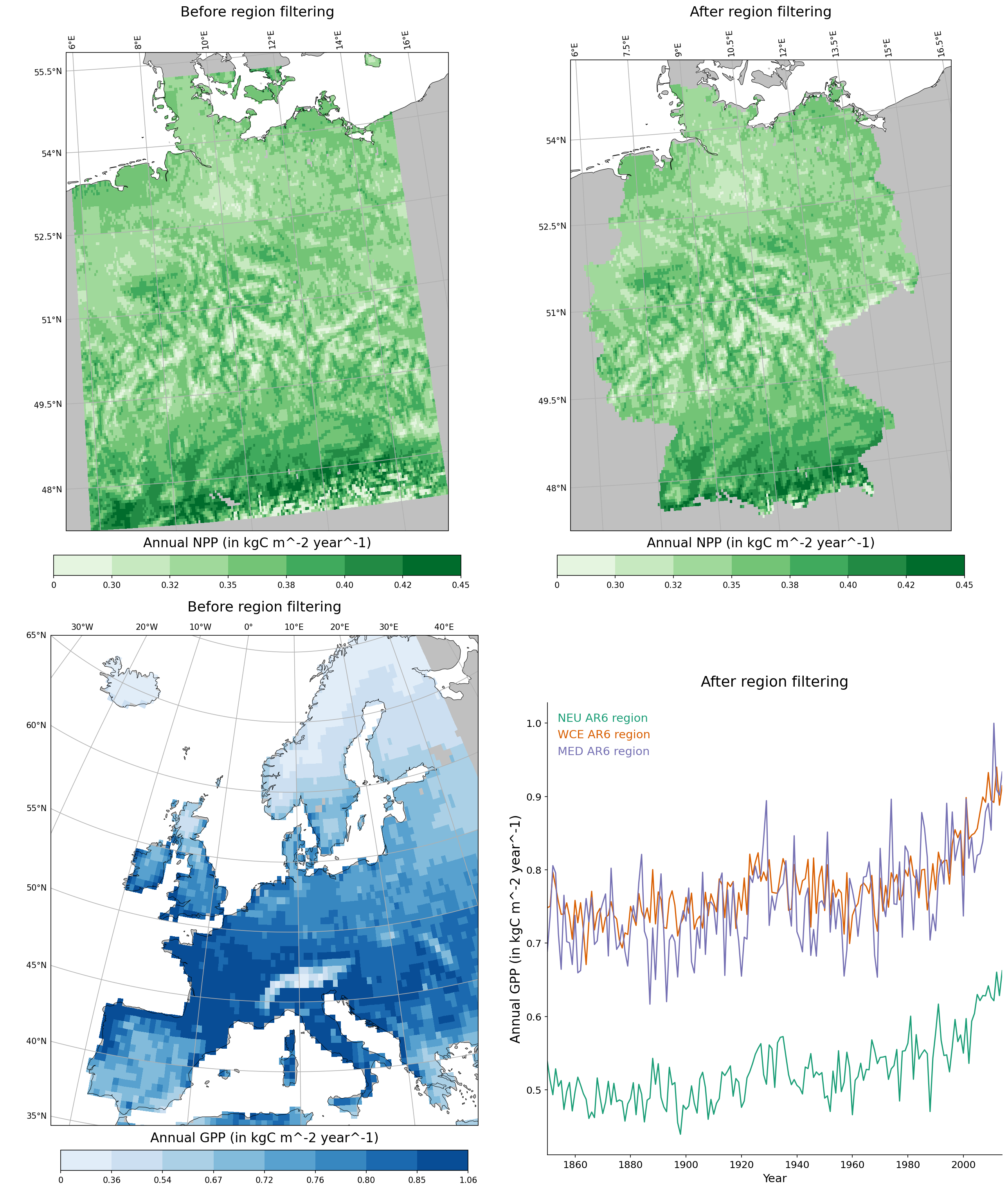
Selecting a geographical region
The method Field.select_region() lets you subset a field to only retain grid cells whose coordinates fall inside a named geographical region. Regions can come from different predefined sets via the region_type argument:
country: Natural Earth countries (10m² resolution); see Natural Earth: Admin 0 – Countriesgiorgi: Giorgi climate regions; see Giorgi & Francisco (2000)SREX: IPCC SREX regions; see IPCC DDC AR5 RegionsAR6: IPCC AR6 regions (subregions); see IPCC-WG1 Atlas reference regions
Here are two examples, (1) select a field to Germany and (2) select another field to 3 IPCC AR6 European subregions and compare time-series:
import canopy as cp
import canopy.visualization as cv

# Germany example

npp_ger_path = "example_data/germany/anpp.out.gz"

npp_ger = cp.Field.from_file(npp_ger_path, file_format="lpjg_annual", grid_type="lonlat", source="lpjguess:anpp")

filtered_npp_ger = npp_ger.select_region("Germany")

fig1 = cv.make_simple_map(field=npp_ger, layer="Total", title="Before region selection", classification=[0,0.3,0.325,0.35,0.375,0.4,0.425,0.45], palette="Greens", proj="AlbersEqualArea", return_fig=True)

fig2 = cv.make_simple_map(field=filtered_npp_ger, layer="Total", title="After region selection", classification=[0,0.3,0.325,0.35,0.375,0.4,0.425,0.45], palette="Greens", proj="AlbersEqualArea", return_fig=True)

# Europe example

gpp_eu_path = "example_data/david/agpp.out"

gpp_eu = cp.Field.from_file(gpp_eu_path, file_format="lpjg_annual", grid_type="lonlat", source="lpjguess:agpp")

neu_gpp_eu = gpp_eu.select_region("NEU", "ar6")
wce_gpp_eu = gpp_eu.select_region("WCE", "ar6")
med_gpp_eu = gpp_eu.select_region("MED", "ar6")

fig3 = cv.make_simple_map(field=gpp_eu, layer="Total", title="Before region selection", n_classes = 8, classification = "quantile", palette="Blues", proj="EuroPP", force_zero=True, return_fig=True)

fig4 = cv.make_time_series(fields=[neu_gpp_eu,wce_gpp_eu,med_gpp_eu], gridop="av", layers="Total", field_labels=["NEU AR6 region", "WCE AR6 region", "MED AR6 region"], title="After region selection", legend_style="highlighted", palette="Dark2", return_fig=True)

cv.multiple_figs([fig1,fig2,fig3,fig4], output_file="filter_region.png")
Changing the units
The units of a Field can be changed with the Field.convert_units() method, which takes three arguments:
factor: The multiplicative factor to apply.units: The new units (a string).inplace: IfTrue, the unit change is performed in place. IfFalse, a new field with the new units is created and returned.
# Change evapotranspiration units from mm to m
print("Before unit change:")
print(aaet)
print(aaet.data)
aaet.convert_units(1.e-3, 'm', inplace=True)
print("After unit change:")
print(aaet.data)
Before unit change:
Data
----
name: Annual AET
units: mm
description: Annual actual evapotranspiration by PFT
file format: LPJ-GUESS: common output (annual)
original file: /home/belda-d/data/pyguess_test_data/europe_LR_100p/output/aaet.out.gz
source: LPJ-GUESS

Grid: lonlat
------------
Longitude:
-26.25 to 34.75 (step: 0.5)
Latitude:
35.25 to 71.75 (step: 0.5)

Time series
-----------
Span: 1850-01-01 00:00:00 - 2014-12-31 23:59:59.999999999
Frequency: Y-DEC

History
-------
2025-05-13 16:06:19: Data read from /home/belda-d/data/pyguess_test_data/europe_LR_100p/output/aaet.out.gz
                   Abi_alb   BES  Bet_pen  ...  Til_cor  C3_gr   Total
lon    lat   time                          ...
-26.25 69.25 1850      0.0  0.00      0.0  ...      0.0   0.00    0.00
             1851      0.0  0.00      0.0  ...      0.0   0.00    0.00
             1852      0.0  0.00      0.0  ...      0.0   0.00    0.00
             1853      0.0  0.00      0.0  ...      0.0   0.00    0.00
             1854      0.0  0.00      0.0  ...      0.0   0.00    0.00
...                    ...   ...      ...  ...      ...    ...     ...
 34.75 69.25 2010      0.0  0.25      0.0  ...      0.0   1.19  105.49
             2011      0.0  0.27      0.0  ...      0.0   1.28  117.36
             2012      0.0  0.31      0.0  ...      0.0   1.61  136.71
             2013      0.0  0.29      0.0  ...      0.0   1.30  128.72
             2014      0.0  0.29      0.0  ...      0.0   1.28  128.42
After unit change:
Data
----
name: Annual AET
units: m
description: Annual actual evapotranspiration by PFT
file format: LPJ-GUESS: common output (annual)
original file: /home/belda-d/data/pyguess_test_data/europe_LR_100p/output/aaet.out.gz
source: LPJ-GUESS

Grid: lonlat
------------
Longitude:
-26.25 to 34.75 (step: 0.5)
Latitude:
35.25 to 71.75 (step: 0.5)

Time series
-----------
Span: 1850-01-01 00:00:00 - 2014-12-31 23:59:59.999999999
Frequency: Y-DEC

History
-------
2025-05-13 16:06:19: Data read from /home/belda-d/data/pyguess_test_data/europe_LR_100p/output/aaet.out.gz
                   Abi_alb      BES  Bet_pen  Bet_pub  ...  Que_rob  Til_cor    C3_gr    Total
lon    lat   time                                      ...
-26.25 69.25 1850      0.0  0.00000      0.0  0.00000  ...      0.0      0.0  0.00000  0.00000
             1851      0.0  0.00000      0.0  0.00000  ...      0.0      0.0  0.00000  0.00000
             1852      0.0  0.00000      0.0  0.00000  ...      0.0      0.0  0.00000  0.00000
             1853      0.0  0.00000      0.0  0.00000  ...      0.0      0.0  0.00000  0.00000
             1854      0.0  0.00000      0.0  0.00000  ...      0.0      0.0  0.00000  0.00000
...                    ...      ...      ...      ...  ...      ...      ...      ...      ...
 34.75 69.25 2010      0.0  0.00025      0.0  0.00000  ...      0.0      0.0  0.00119  0.10549
             2011      0.0  0.00027      0.0  0.00001  ...      0.0      0.0  0.00128  0.11736
             2012      0.0  0.00031      0.0  0.00001  ...      0.0      0.0  0.00161  0.13671
             2013      0.0  0.00029      0.0  0.00000  ...      0.0      0.0  0.00130  0.12872
             2014      0.0  0.00029      0.0  0.00000  ...      0.0      0.0  0.00128  0.12842
Selecting overlapping entries
When comparing two fields (for example, simulations vs observations, different model runs…) we often need the fields to have matching spatial and temporal coordinates. We can select entries with matching coordinates with the overlap() function, as in the following example:
# This will match field entries with slightly offset spatial coordinates
import canopy as cp

# Load (dummy) data sources:
my_source = cp.get_source("/path/to/some/data", "lpj_guess")
my_other_source = cp.get_source("/path/to/some/other/data", "lpj_guess")

# Load fields
field1 = my_source.load_field('anpp')
field2 = my_other_source.load_field('anpp')

print("Original data:")
print("--------------\n")
print("field1's data:")
print(field1.data)
print("field2's data:")
print(field2.data)

# Exact coordinate matching leads to empty fields in this case:
print()
print("Matching coordinates exactly:")
print("-----------------------------\n")
field1_overlap, field2_overlap = cp.overlap(field1, field2)
print("field1's data after overlap:")
print(field1_overlap.data)
print("field2's data after overlap:")
print(field2_overlap.data)

print()
print("Matching with a spatial coordinate tolerance 0.2 deg.:")
print("------------------------------------------------------\n")
field1_overlap, field2_overlap = cp.overlap(field1, field2, atol=0.2)
print("field1's data after overlap:")
print(field1_overlap.data)
print("field2's data after overlap:")
print(field2_overlap.data)

print()
print("Using field1's coordinates for the returned fields:")
print("---------------------------------------------------\n")
field1_overlap, field2_overlap = cp.overlap(field1, field2, atol=0.2, use_index="left")
print("field1's data after overlap:")
print(field1_overlap.data)
print("field2's data after overlap:")
print(field2_overlap.data)

print()
print("Using field2's coordinates for the returned fields:")
print("---------------------------------------------------\n")
field1_overlap, field2_overlap = cp.overlap(field1, field2, atol=0.2, use_index="right")
print("field1's data after overlap:")
print(field1_overlap.data)
print("field2's data after overlap:")
print(field2_overlap.data)
Original data:
--------------

field1's data:
              TrBE  C4G
lon lat time
1.0 1.0 1989     0    0
        1990     1    2
    2.0 1989     2    4
        1990     3    6
2.0 3.0 1989     4    8
        1990     5   10
        1991     6   12
field2's data:
               TrBE  C4G
lon lat  time
1.1  2.1 1990     1    2
2.1  3.1 1990     3    4
         1991     5    6
         1992     7    8
3.1 -3.1 1984     9   10

Matching coordinates exactly:
-----------------------------

field1's data after overlap:
Empty DataFrame
Columns: [TrBE, C4G]
Index: []
field2's data after overlap:
Empty DataFrame
Columns: [TrBE, C4G]
Index: []

Matching with a spatial coordinate tolerance 0.2 deg.:
------------------------------------------------------

field1's data after overlap:
              TrBE  C4G
lon lat time
1.0 2.0 1990     3    6
2.0 3.0 1990     5   10
        1991     6   12
field2's data after overlap:
              TrBE  C4G
lon lat time
1.1 2.1 1990     1    2
2.1 3.1 1990     3    4
        1991     5    6

Using field1's coordinates for the returned fields:
---------------------------------------------------

field1's data after overlap:
              TrBE  C4G
lon lat time
1.0 2.0 1990     3    6
2.0 3.0 1990     5   10
        1991     6   12
field2's data after overlap:
              TrBE  C4G
lon lat time
1.0 2.0 1990     1    2
2.0 3.0 1990     3    4
        1991     5    6

Using field2's coordinates for the returned fields:
---------------------------------------------------

field1's data after overlap:
              TrBE  C4G
lon lat time
1.1 2.1 1990     3    6
2.1 3.1 1990     5   10
        1991     6   12
field2's data after overlap:
              TrBE  C4G
lon lat time
1.1 2.1 1990     1    2
2.1 3.1 1990     3    4
        1991     5    6
Combining fields
Fields can be combined in two main ways:
Unite fields: combine fields along the spatial and/or temporal axes.
Join fields: combine fields with non-overlapping layers into a single field.
Unite
A unite() operation combines fields along the spatial and/or temporal axes. The fields to unite must fulfill the following requirements:
Their time series must have the same frequency
Their grids must be of the same type and compatible (see documentation for grid compatibility)
All fields must have at least one overlapping layer
Additionally, we can instruct unite() to perform several optional checks on the fields’ data before uniting them by using the checks argument:
't': check that fields identical time series'c': check that fields have contiguous time series'g': check that all gridcells overlap between fields'd': (disjoint) check that there are no common gridcells
:func’unite returns a single field with only the common layers among the passed fields.
A possible use case is combining the outputs of simulations covering different spatial domains (for example, if you had to break up a big simulation into several pieces and now need to put the outputs together):
import canopy as cp

# Uniting pieces of a simulation broken down into smaller spatial domains
# -----------------------------------------------------------------------
anpp1 = cp.Field.from_file('/path/to/run1/anpp.out', source='lpjguess:anpp')
anpp2 = cp.Field.from_file('/path/to/run2/anpp.out', source='lpjguess:anpp')
anpp3 = cp.Field.from_file('/path/to/run3/anpp.out', source='lpjguess:anpp')

# In this case we might want to check that the time series of all the pieces are the same
# and that the fields do not overlap spatially
anpp = cp.unite([anpp1, anpp2, anpp3], checks='td')
Another use case is concatenating a historical run with a scenario run (uniting along the time axis).
import canopy as cp

aaet_hist = cp.Field.from_file('/path/to/historical/run/aaet.out')
aaet_ssp126 = cp.Field.from_file('/path/to/ssp126/run/aaet.out')

# In this case we might want to check that there are no missing gridcells
# between the 2 runs and that the time series connect with no gaps
aaet_full2 = cp.unite([aaet_hist, aaet_ssp126], chekcs = 'cg')
Join
A join() operation combines fields along the “layers axis”. The most common use case for this is to join several fields from the same simulation into a single field. The fields to unite must fulfill the following requirements:
Their time series must have the same frequency
Their grids must be of the same type and compatible
Fields have no overlapping layers
join() returns a single field with all the layers from the original fields. Entries with non-overlapping spatio-temporal coordinates are completed with NaNs.
't': check that fields have identical time series'g': check that all gridcells overlap between fields'i': check that indices are identical (supersedes both checks above)
import canopy as cp

mgpp = cp.Field.from_file("/path/to/montlhy/output/mgpp.out")
mnpp = cp.Field.from_file("/path/to/monthly/output/mnpp.out")
mnee = cp.Field.from_file("/path/to/monthly/output/mnee.out")

# Let's combine all these into a single field:
monthly_fluxes = cp.join([mgpp, mnpp, mnee])